9. Source Convergence Diagnosis and Acceleration
Monte Carlo criticality calculation uses fission source iteration method. The convergence speed of fission source distribution depends on the system dominance ratio. For systems with high dominance ratio (such as full reactor and spent fuel pool), fission source convergence may take hundreds or even thousands of generations, resulting in a lot of computing time wasted on inactive generations that do not directly contribute to the statistical results.
9.1. Shannon Entropy and Progressive Relative Entropy Statistics
The RMC source convergence module provides Shannon Entropy statistical function, which qualitatively reflects the convergence trend of fission source distribution and helps users choose a reasonable number of inactive generation neutrons.
Shannon entropy is defined as:
where \(S(i)\) is the fission source fraction of the \(i\) th mesh cell.
The RMC source convergence module also provides a progressive relative entropy (PRE) statistical function. Similar to the Shannon entropy function, PRE can qualitatively reflect the convergence trend of the fission source distribution and help users choose a reasonable number of inactive generation neutrons.
The relative entropy is defined as:
where \(S\) and \(Y\) are fission source distributions, \(S(i)\) and \(Y(i)\) are the fission source fraction of the \(i\) th mesh cell. \(D(S||Y)\) is always non-negative, and when \(S = Y\) , \(D(S||Y) = 0\).
Shannon entropy can characterize the disorder of source distribution, while relative entropy characterizes the deviation between two source distributions. The larger the relative entropy, the greater the deviation, and the smaller the similarity between the two source distributions. The relative entropy may be infinite, so the quantity that better characterizes the deviation between two source distributions is the progressive relative entropy PRE. PRE is defined as:
where \(S^{(j)}\) is the fission source distribution of the \(j\) th iteration step.
Shannon entropy or progressive relative entropy is defined by the following input card:
SeMesh [Scope = < xNum yNum zNum >]
[Bound = <xMin xMax yMin yMax zMin zMax>]
[PRE = <flag>]
[Output = <flag>]
where,
- SeMesh is the keyword for the Shannon Entropy Mesh input option.
- Scope specifies the number of divisions in the Shannon entropy mesh in the x, y, and z directions. xNum , yNum , and zNum are positive integers.
- Bound specifies the boundary range of the Shannon entropy mesh in the x, y, and z directions. If the number of mesh divisions in a certain direction is specified as -1 in the Scope input option, the default mesh boundary is (-∞, +∞), and the boundary of the corresponding direction in Bound has no practical meaning. *Note that the user should ensure that the mesh range can cover the neutron tracking area, otherwise the statistical results of the Shannon entropy will be incorrect.*
- PRE specifies whether to calculate the progressive relative entropy. When PRE = 1 , the progressive relative entropy is calculated; when PRE = 0 , the progressive relative entropy is not calculated (default value). Note that the program can only calculate Shannon entropy or progressive relative entropy, not both.
- Output specifies whether to output the neutron source fractions in the mesh. When Output = 0 (default), no neutron source fractions are output; when Output = 1 , the neutron source fractions for each generation are output to the convergence/source data set in the .Info.h5 file, and each generation of data sets is named after the generation.
9.2. Statistics of the coefficients of the fission source distribution functional expansion
The RMC source convergence module provides the function of statistical functional expansion coefficients to characterize the shape of fission source distribution, qualitatively reflects the change of fission source distribution shape with iteration steps, and helps users choose a reasonable number of inactive generation neutrons.
The function is defined by the following input options:
FET [Axis = <x y z>]
[Bound = <x_boundary_min x_boundary_max y_boundary_min y_boundary_max z_boundary_min z_boundary_max>]
where,
- FET is the keyword for input card for the function.
- Axis specifies the coordinate axis of the fission source distribution shape. The program only allows the use of functional expansion coefficients to characterize the fission source distribution shape from the three coordinate axes of the Cartesian coordinate system, namely, x, y, and z. For example, if the functional expansion coefficients in the x and z directions are needed to characterize the fission source distribution shape, you need to specify Axis = 1 0 1 .
- Bound specifies the boundary range of the fission source distribution shape in three directions. The boundary range needs to be larger than the positions where all neutrons may undergo fission reactions, and the smaller the better. Note that boundary_min < boundary_max . When statistics in a certain direction are not needed, the relevant values can be arbitrary. For example, if the functional expansion coefficients in the x and z directions are needed to characterize the fission source distribution shape, you can specify Bound = -300 300 0 0 0 300 .
It should be noted that this option is not compatible with the fission source convergence acceleration methods (such as asymptotic Wieland, asymptotic hyperhistory method).
9.3. Fission Matrix Statistics
The RMC source convergence module also provides fission matrix statistics. Based on the fission matrix, Monte Carlo undersampling can be diagnosed and the dominance ratio can be calculated. In addition to using the fission matrix to calculate the dominance ratio, RMC also supports the dominance ratio calculation method based on the error transfer matrix, which is not available in the current version.
The fission matrix is defined as follows: Each element \(F_{ij}\) in the fission matrix F indicates the probability of neutrons born in area \(j\) undergoing fission to produce neutrons in area \(i\).
The input format of the fission matrix statistics input option is similar to the Shannon entropy statistics card:
FmMesh [Scope = < xNum yNum zNum >]
[Bound = <xMin xMax yMin yMax zMin zMax>]
where,
- FmMesh is the keyword for the fission matrix mesh input option.
- Scope specifies the number of mesh divisions of the Shannon entropy mesh in the x, y, and z directions. xNum , yNum , and zNum are positive integers. The size of the fission matrix is (xNum *yNum*zNum)2, and if the mesh division is too fine, the calculation efficiency may be reduced.
- Bound specifies the boundary range of the Shannon entropy mesh in the x, y, and z directions. If the number of mesh divisions in a certain direction is specified as -1 in Scope , the default mesh boundary is (-∞, +∞), and the boundary of the corresponding direction in Bound has no practical meaning. Note that the user should ensure that the mesh range is able to cover the neutron tracking area, otherwise the statistical results of the fission matrix will be wrong.
9.4. Source Convergence Acceleration
RMC uses the asymptotic hyperhistory method and the asymptotic Weiland method to accelerate source convergence and reduce the number of inactive generations. The current version only provides the asymptotic hyperhistory acceleration method.
The input options for the source convergence acceleration function are:
AcceFsc [Factor = <f(1) p(1) f(2) p(2) …f(n) p(n)>]
        [AutoFactor = <inactive_cycle>]
where,
- AcceFsc is the keyword for the Shannon Entropy Mesh Input Card.
- Factor and AutoFactor are used to specify the parameters of the asymptotic hyperhistory acceleration method and will be discussed separately later.
9.4.1. Factor Input Option
Factor is used to customize the acceleration parameters. The f(i) in the input card is called the acceleration factor, and p(i) is called the acceleration period. Its meaning is: in the first p(1) generation, use the acceleration factor f(1); in the next p(2) generation, use the acceleration factor f(2); and so on. The principle of the asymptotic superhistorical acceleration method is not introduced in detail here, only the two parameters of the acceleration factor and the acceleration period are introduced as follows:
The larger the acceleration factor f(i), the more obvious the acceleration effect is, but the statistical fluctuation may also be greater. The user needs to define a set of asymptotically decreasing acceleration factors {f(i)}, such as “16 → 8 → 4 → 2”. Note that the acceleration factor should not be too large (it is recommended to be less than 20), otherwise it may cause instability.
The acceleration period p(i >1) is generally set to 5-10 generations. The first acceleration period p(1) is usually set larger because it corresponds to the largest acceleration factor and plays a major role in the acceleration effect.
The asymptotic hyperhistory acceleration method acts on the first few inactive generations, and the acceleration effect it produces is roughly equivalent to the time taken to compute all inactive generations without acceleration. For example, a full-reactor critical calculation requires about 200 inactive generations without acceleration. By using “factor = 16 10 8 5 4 5 2 5” to accelerate the first 10+5+5+5=25 inactive generations, a basically equivalent convergence effect as computing 200 non-accelerated inactive generations can be achieved.
9.4.2. AutoFactor Input Option
As an alternative to Factor , the RMC program provides AutoFactor for automatically generating source convergence acceleration parameters. For ordinary users, it is recommended to use AutoFactor instead of the custom input in Factor . In AutoFactor , the user specifies the number of inactive generations when the acceleration method is not used (inactive_cycle), and the program will automatically generate the parameter sequence of the asymptotic hyperhistory method. Assuming that the number of inactive generations when the acceleration method is not used is N, the required number of inactive generations after using AutoFactor is approximately:
For example, a full-reactor calculation requires 300 generations to converge. After using automatic source convergence acceleration, the required inactive generations can be set to: \(N' = \frac {300}{16} + 15 \approx 35\). If the number of inactive generations N specified in AutoFactor is less than 30, the program will turn off the source convergence acceleration function.
9.4.3. Notes on Source Convergence Acceleration
When using the source convergence acceleration method, reasonable matching parameters should be used in the PowerIter input option of the criticality calculation module, including:
1)Specify a reasonable initial effective multiplication factor in Keff0 to allow the final result to be close to the true Keff.
2)Specify a sufficiently large number of particles per generation in Population . For full-reactor criticality calculations, it is recommended that the number of particles per generation be greater than 100,000.
3)Specify a reasonable number of inactive generations in Population . The number of inactive generations should be greater than or equal to the source convergence acceleration number.
9.5. Source Convergence Module Input Example
9.5.1. Acceleration of OECD benchmark source convergence
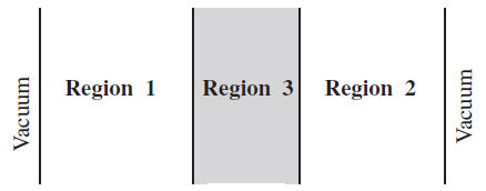
图9.2 OECD Monte Carlo source convergence benchmark problem
图9.2 describes a benchmark problem in the OECD Monte Carlo source convergence study. The benchmark problem is a weakly coupled system consisting of three 1D plates, with 20 cm thick fuel zones on both sides and a 30 cm water layer in the middle. The initial source position is located at the center of the fuel zone on the left. The number of inactive generations required for conventional source iteration convergence is about 1000. Through the RMC source convergence acceleration method, the number of inactive generations can be reduced to less than 100. In the source convergence module of 示例9.3, the number of Shannon entropy mesh cells is specified to be 70 and the width is 1.0 cm. This example requires a large number of particles to be simulated, and it is recommended to use a parallel machine to complete the calculation.
///// OECD MC convergence benchmark 3 . SHE Ding 2012-09-12 /////
UNIVERSE 0
cell 1 1 & -2 mat = 1
cell 2 2 & -3 mat = 2
cell 3 3 & -4 mat = 1
cell 4 -1 : 4 void = 1

SURFACE
surf 1 px 0
surf 2 px 20
surf 3 px 50
surf 4 px 70

MATERIAL
mat 1 9.9487E-02
      92235.30c 7.6864E-05
      92238.30c 6.8303E-04
      8016.30c 3.7258E-02
      1001.30c 5.9347E-02
      7014.30c 2.1220E-03
mat 2 1.0006E-01
      1001.30c 6.6706E-02
      8016.30c 3.3353E-02

CRITICALITY
PowerIter population = 500000 100 1000
InitSrc point = 10 0 0

Tally
Celltally 1 type = 1 cell = 1 3

CONVERGENCE
SeMesh Scope = 70 -1 -1 Bound = 0 70 0 1 0 1
FmMesh Scope = 70 -1 -1 Bound = 0 70 0 1 0 1
AcceFsc Autofactor = 1000
9.5.2. Hoogenboom Full-Reactor Benchmark Source Convergence Acceleration
示例9.4 describes the Hoogenboom Monte Carlo full-reactor benchmark. The number of inactive generations required for the conventional source iteration to converge is about 250. By using the automatic source convergence acceleration parameter, the number of inactive generations is set to 35. In the source convergence input module, a Shannon entropy mesh (21×21) based on the component is defined to help the user diagnose the source convergence trend. This example requires a large number of particles to be simulated, and it is recommended to use a running machine capable of parallelization to complete the calculation.
// same model as previous

CONVERGENCE
SeMesh Scope = 21 21 1 Bound = -224.91 224.91 -224.91 224.91 -229 223
AcceFsc Autofactor = 250